Elimination with matrices

• We use it to find solution of linear equations
  • Elimination method is also popular among software packages like Matlab.
• We would perform row operations to make matrix upper triangular
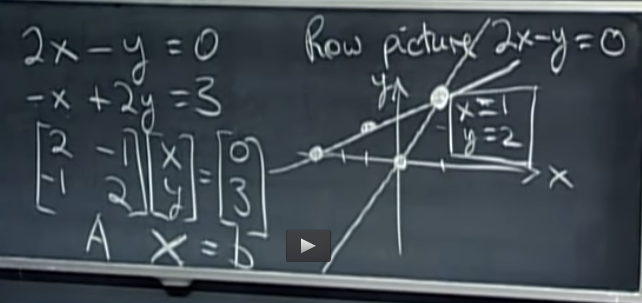
• We can do this with equations itself (without putting in matrix)
  • We don’t want to keep writing variable names
• Process
  • Iteratively select diagonal element as pivot
  • Make all entires below it 0
  • Repeat
• Allowed row operations are the ones which does not change systems
  • Switching rows
  • Multiplying row with constant
  • Add rows

What would happen when we have 2 variable and 100 equations (observation) ?

• Here are four terms
  • Underdetermined System (no of equation > no of unknowns)
  • Overdetermined system (no of equation < no of unknowns)
  • Consistent System (one/more set of values satisfy equations)
  • Inconsistent System (no set of values satisfy equations)
• Overdetermined system is generally inconsistent except
  • Same equation multiplied by constant
  • One equation is linear combination of other
• More specifically, according to the Rouché–Capelli theorem, any system of linear equations (underdetermined or otherwise) is inconsistent if the rank of the augmented matrix is greater than the rank of the coefficient matrix.

Snippets for Prof Gilbert’s course

Elimination matrices – we can create matrix for each elimination operation

Remember – Multiply on left is row operation, multiply on right is column operation

Permutation matrix (P) – Exchange the rows of identity matrix

It is easy to find inverse of this elimination matrices

Reference

These are notes from Prof. Gilbert Strang’s lecture on MIT open courseware. https://ocw.mit.edu/courses/mathematics/18-06-linear-algebra-spring-2010/video-lectures/lecture-1-the-geometry-of-linear-equations/

Geometry of Linear Equations – Column Picture

Notes from Prof. Gilbert Strang’s Lecture on MIT OpenCourseWare: The Geometry of Linear Equations

In linear algebra, when faced with equations, we often try to visualize them using the row picture.

Row Picture: In 2-D, we can think of it as a line and aim to find its intersection.

Column Picture: We aim to find the weights of a linear combination of columns. In the image on the right, we see the addition of two vectors. We start from the origin and add them at the tail.

As we move to higher dimensions, the row picture becomes more challenging to visualize, while the column picture remains straightforward.

Furthermore, the column picture allows us to check if the combination of all columns fills the entire space. We can verify this through elimination.

Additionally, we can develop a habit of viewing matrix multiplication as a linear combination of columns.