This post serves as a lecture summary of a course offered by the University of Washington, which can be accessed at the following link: University of Washington – ML: Clustering and Retrieval.
Sample code related to the course can be found on GitHub at: Sample Code for EM Algorithm.
In this lecture, we will cover several important topics:
- Why we need probabilistic clustering: We will explore the motivations behind using probabilistic clustering methods, which allow for soft assignments to clusters rather than rigid assignments.
- Mixture models: We will dive into the concept of mixture models, which are a probabilistic approach to clustering. Mixture models allow data points to belong to multiple clusters with different probabilities.
- Expectation Maximization (EM): We will study the Expectation Maximization algorithm, a powerful iterative algorithm used to estimate the parameters of mixture models. EM alternates between the expectation step, where cluster assignments are updated based on current parameter estimates, and the maximization step, where the parameters are updated based on current cluster assignments.
Why we need probabilistic clustering ?
To understand the need for probabilistic clustering, let’s consider the problem of determining user preferences based on their feedback. Suppose users provide feedback on whether they liked or disliked an article. We want to gather this feedback and group it into clusters to gain insights into their preferences.
For instance, imagine a user who likes an article about the first human landing on Mars. This article could be relevant to both world news and science news categories. In such cases, assigning articles to clusters with a hard assignment (where an article belongs to only one cluster) may not capture the complete picture. Soft assignment to clusters, where an article can belong to multiple clusters with different probabilities, is more suitable.
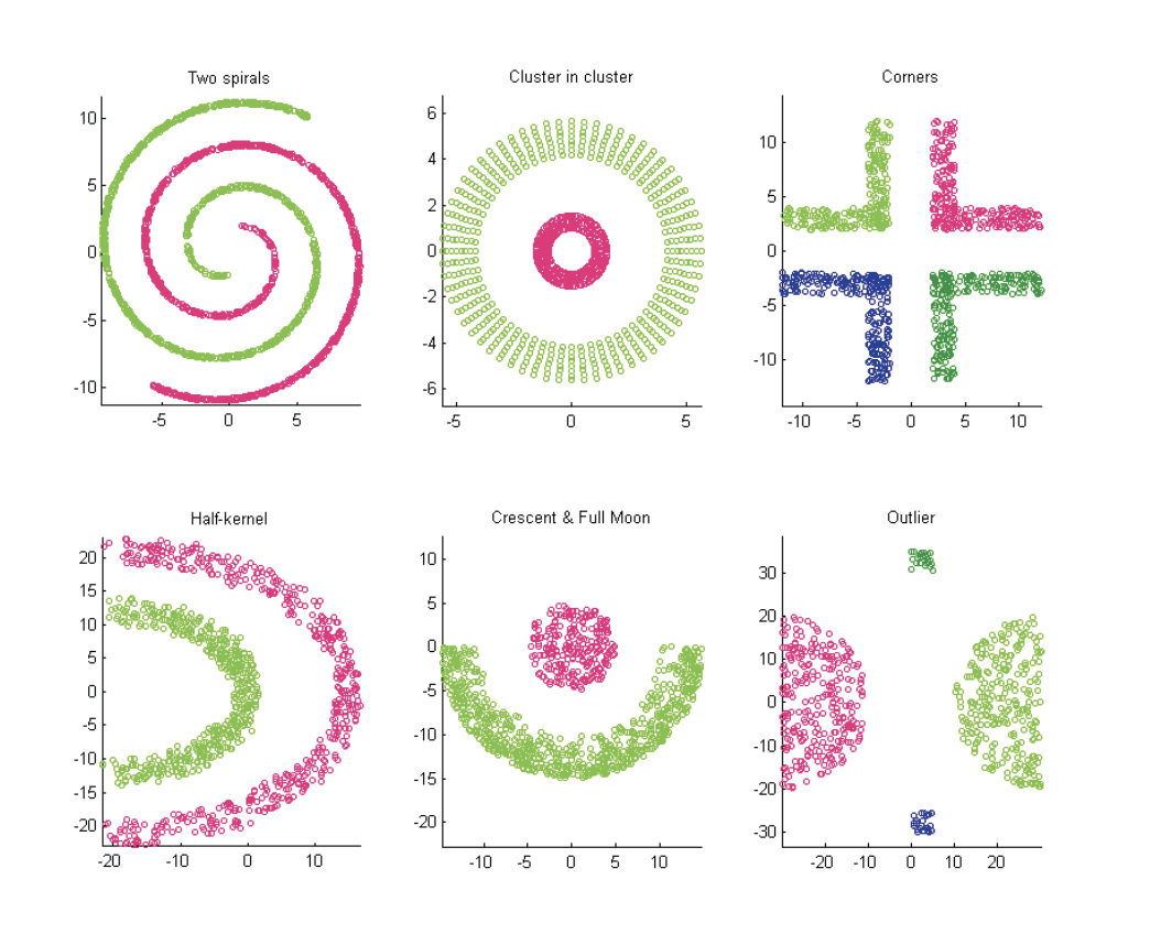
Now, let’s explore some scenarios where the traditional K-means algorithm fails:
- Clusters with Different Spreads: When clusters have varying spreads, simply deciding based on a single sample may not provide an accurate representation. Instead, it is important to consider the number of data points within each cluster. Assigning an ambiguous point to a cluster that has more data points can be a more meaningful approach.
- Overlapping Clusters: In cases where clusters overlap, soft assignment becomes crucial. It allows for assigning data points to multiple clusters based on the degree of membership.
- Clusters with Different Shapes or Orientations: When clusters have distinct shapes or orientations, measuring the distance to the cluster center alone is insufficient. Considering the shape of the clusters is necessary for accurate clustering.
One approach to address these challenges is using K-means with scaled Euclidean distance. This modification results in clusters represented by axis-aligned ellipses, accommodating different spreads in each dimension. However, determining appropriate weights for each dimension in the calculation remains a question that needs to be addressed. Shape is still axis-aligned ellipses, which is a limitation in itself.
Motivating application
Let’s consider the task of clustering images based on their color composition. One approach is to compute the average values of the red (R), green (G), and blue (B) channels for each image. This results in representing each image as a single 3-dimensional vector [R, G, B], capturing the average color values.
By applying clustering algorithms to these image vectors, we can group similar images together based on their dominant color characteristics. Although our data is unlabeled, we can observe potential clusters such as:
- Sky Cluster (Blue Dominated): Images that predominantly contain blue colors, such as those depicting clear skies, can be grouped into this cluster.
- Sunset Cluster (Red Dominated): Images showcasing vibrant sunsets with warm hues and red tones can be grouped into this cluster.
- Forest Cluster (Green Dominated): Images featuring lush green forests, landscapes, or vegetation will likely be grouped into this cluster due to their dominant green color composition.
Mixture Models
- Here is how distribution of blue might look for all images
We can model image clustering using a mixture of Gaussian distributions. The model consists of three Gaussian components, each with its own parameters (μ and σ). The final distribution is a convex combination of these components: π1g1 + π2g2 + π3*g3, where 0 ≤ π ≤ 1 and the sum of all π values is equal to 1.
Each mixture component represents a unique cluster, characterized by its own set of parameters (πk, μk, σk). In the case of multidimensional data, such as image vectors, each individual distribution is a multivariate Gaussian distribution.
Without examining the image vector, we can determine the probability of it belonging to cluster k using the πk value. Given an image vector x, we can estimate the probability of it belonging to cluster k as P(x | params) = P(x | μk, Σk), where Σ represents the covariance matrix in the multivariate Gaussian.
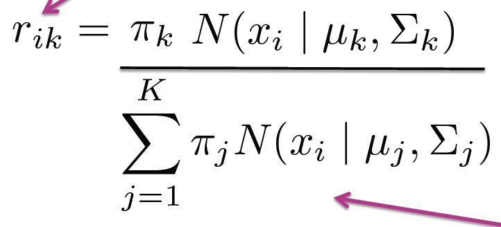
Clustering with soft assignment involves calculating a responsibility vector for each data point. The length of the responsibility vector corresponds to the number of clusters, which in this case is three (sky, forest, sunset). Each element of the responsibility vector represents the probability of a data point belonging to a specific cluster.
In the case of document clustering, where the dimensionality is high (proportional to the number of words in a vocabulary), keeping track of parameters for each Gaussian becomes computationally expensive. To address this, we simplify the model by considering only diagonal values in the covariance matrix, effectively restricting the model to axis-aligned ellipses. This approach is similar to K-means with scaled Euclidean distance, which also allows for axis-aligned ellipses.
However, the advantage of the mixture model is twofold:
- We do not need to specify weights for each dimension in advance; the model learns them from the data.
- Different clusters can have varying weights for each dimension, allowing for more flexible modeling of the data.
EM
Responsibility vector calculation with known cluster parameters
- The responsibility vector can be calculated if we know the cluster parameters: π_k, μ_k, and ∑_k.
- The responsibility vector is different from the π values.
- Given a data point, we can find its corresponding responsibility vector by estimating the probabilities in that cluster.
- The responsibility vector needs to be normalized after evaluating the probabilities.
- This process is a consequence of Bayes’ rule.
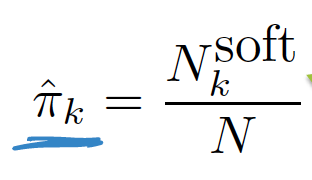
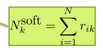
Estimating cluster parameters with known responsibility vectors
- It is similar to parameter estimation of a multivariate Gaussian.
- Each data point, x_i, is multiplied, and there is no need to worry about the denominator since it is also not N (the number of data points).


- N_k_soft implies how many points belong to cluster 1
- Also it is a soft assignment
EM Algorithm
- E-step: Estimation of the responsibility vector given parameters.
- M-step: Maximum likelihood estimation of the parameters given the responsibility vector.
- These two steps are repeated until convergence.
- The EM algorithm can be derived as a coordinate ascent algorithm and converges to a local mode.
- The biased coin example provides a good illustration of the EM algorithm. Check the image below
Challenges
- The probability becomes infinite when the variance becomes zero.
- This can occur when there is only one data point in a cluster, and the mean is itself with zero variance.
- In high-dimensional spaces, this often happens, such as when a document does not have a specific word at all.
- To solve this issue, a small value is added to the diagonal elements of the covariance matrix, similar to adding a prior in Bayesian approaches.
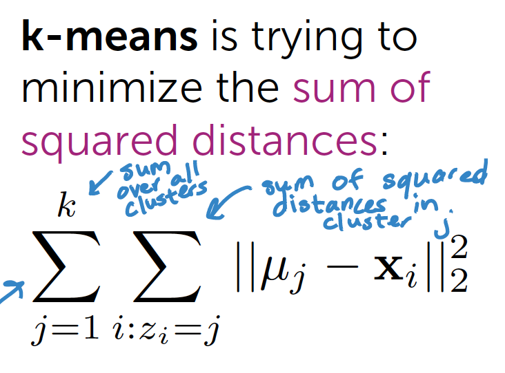
Relationship to K-means:
- When a Gaussian has the same variance in all dimensions and shrinks to zero, the likelihood becomes either 0 or 1.
- This behavior is similar to hard assignment, resembling the K-means algorithm.
Initialisation
- Choose k observations at random and assign observations to nearest centroid
- Above via k-means++
- Solution of k-means
- Grow mixture model by splitting cluster (sometime merging) until K clusters are formed
I have coded simple EM at [0]
References
[0] : https://github.com/arcarchit/datastories/blob/master/EM.ipynb


